Using Homography for Pose Estimation in OpenCV | by Abhinav Peri | Analytics Vidhya | Medium
| Created | |
|---|---|
| Tags | |
| URL | https://medium.com/analytics-vidhya/using-homography-for-pose-estimation-in-opencv-a7215f260fdd |
Photo by ShareGrid on Unsplash
Introduction to Homography
Hello! Our names are Abhinav and Unnathi Peri. We are students at Westlake High School who participate on our FRC robotics team, 2687 Team Apprentice. Our goal with this project was to be able to find out where we were relative to certain patterns on the field to know our global position during the game. Hopefully through this article, we can share what we learned for others to benefit.
What is Homography
Homography is a planar relationship that transforms points from one plane to another. It is a 3 by 3 matrix transforming 3 dimensional vectors that represent the 2D points on the plane. These vectors are called Homogeneous coordinates, and are discussed below. The illustration below represents the relationship; the 4 points correspond between the red plane and the image plane. Homography stores the position and orientation of the camera and this can be retrieved by decomposing the homography matrix.
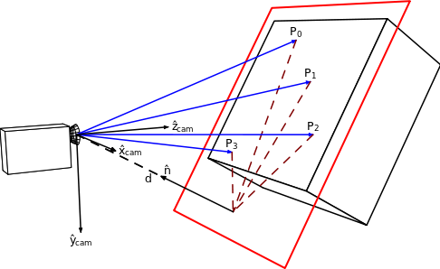
https://en.wikipedia.org/wiki/File:Homography-transl-bold.svg
Pinhole Camera
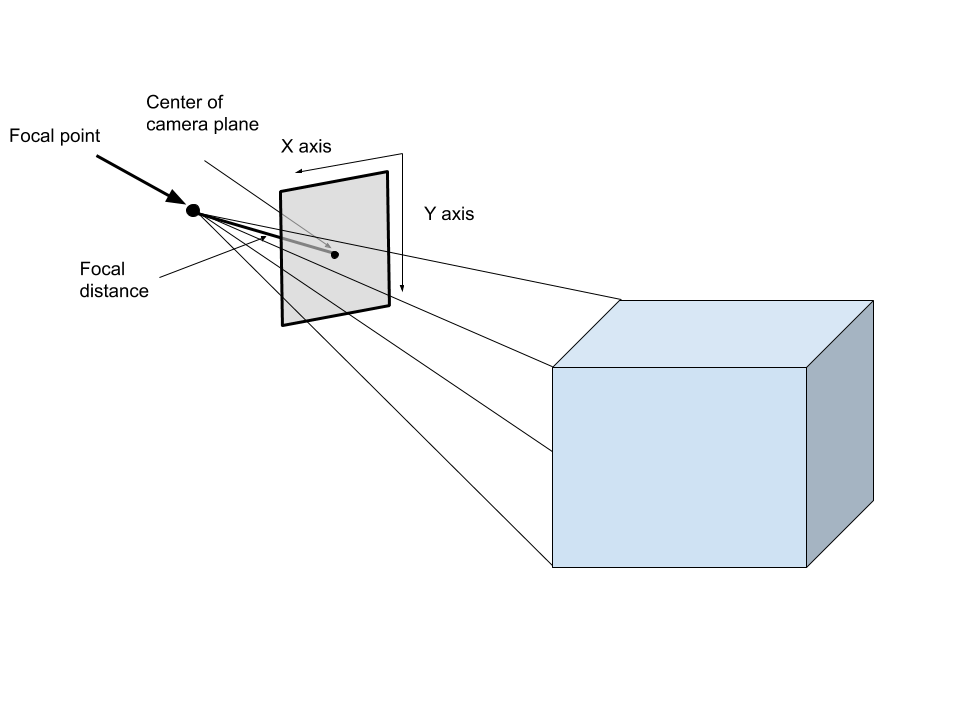
Pinhole Camera Model (Explained below)
The pinhole camera model is a mathematical representation of a camera. It takes in 3D points and projects them onto an image plane like the illustration above. Some important aspects of the model are the focal point, the image plane(gray plane in the image above), the principal point (The bolded dot on the image plane in the image above), the focal length (distance between the image plane and the focal point), and the optical axis (The line perpendicular to the image plane that goes through the focal point). This transformation can be encoded in a Projection Matrix, which transforms 4 dimensional homogeneous vectors representing 3D points to 3 dimensional homogeneous vectors representing 2d points on the image plane.
Homogeneous Coordinates
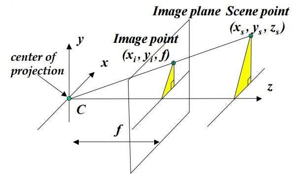
Homogeneous coordinates are projective coordinates that represent points within computer vision. Since there is a conversion from 3D to 2D when taking a picture, the scale of depth is lost. Therefore, an infinite amount of 3D points can be projected to the same 2D point, making homogeneous coordinates very versatile in describing the ray of possibilities since they are similar by scale. Homogeneous coordinates simply take the normal cartesian coordinates, and augment a dimension to the end.
Cartesian coordinates represented in homogeneous coordinates
Homogeneous coordinates are also equivalent by scale.
Coordinates are equal since they only differ through scale
Notice how the triangle could be further away and larger, but it still could produce the same image
Given a homogeneous coordinate, divide all elements by the last element of the vector (scale factor), and then the cartesian coordinate is a vector composing of all the elements except the last.
Projection matrix
The Projection Matrix is a multiplication of 2 other matrices that are related to the camera properties. They are the Extrinsic and Intrinsic camera matrices. These matrices store the extrinsic parameters and the intrinsic parameters of the camera respectively (hence the names).
Projection Matrix (3 by 4 matrix)
Extrinsic Matrix
The extrinsic matrix stores the position of the camera in global space. This information is stored in a rotation matrix as well as a translation vector. The rotation matrix stores the camera’s 3D orientation while the translation vector stores its position in 3D space.
Rotation Matrix
The rotation matrix and the translation vector are then concatenated to create the extrinsic matrix. Functionally, the extrinsic matrix transforms 3D homogeneous coordinates from the global to the camera coordinate systems. Therefore, all transformed vectors will represent the same position in space relative to the focal point.
Intrinsic Matrix
The intrinsic matrix stores the camera intrinsics such as focal length and the principal point. The focal length (fₓ and fᵧ) is the distance from the focal point to the image plane which can be measured in pixel-widths or pixel-heights (hence why there are 2 focal lengths). Each pixel is not a perfect square, so each side has different side lengths. The principal point (cₓ and cᵧ) is the intersection of the optical axis and the image plane (functional center of the image plane). This matrix transforms 3D coordinates relative to the focal point onto the image plane; think of it as the matrix that takes the picture. When combined with the Extrinsic Matrix, the pinhole camera model is created.
Pinhole Camera Model
Now homography is a special case of the pinhole camera model where all the real world coordinates that are projected onto the camera are lying on a plane where the z coordinate is 0. Here is a derivation for Homography.
Derivation of Homography
Pinhole Camera Model
Expanding the Projection Equation with z = 0
Definition of matrix multiplication
Removing redundant information about z values
Definition of Homography matrix

H is the homography matrix, a 3 by 3 matrix that transforms points from one plane to another. Here, the transformation is between the plane where Z = 0 and the image plane that points get projected onto. The homography matrix is usually solved through the 4 point algorithm. Here are some great slides that we used for the math. Essentially, it uses 4 point correspondences from the 2 planes to solve for the homography matrix. In OpenCV, we can find the homography matrix using the method cv2.findHomography:
cv2.findHomography(<points from plane 1>, <points from plane 2>)This method requires some form of feature point tracking so that the results of the method above. The quality of the coordinate measurements will contribute to the accuracy of the method above. Once we have the homography matrix, we can decompose it into translation and rotation of the camera. The decomposition of the homography matrix is shown below:
Decomposition
definition of homography matrix
multiplying by inverse camera matrix
simplifying
normalized solution matrix
We can derive the rotation matrix by taking the first two columns from the solution matrix as the first two columns in the rotation matrix and use a cross product to find the last column of the rotation matrix. The translation is the last column of the solution matrix.
Python Code for Decomposition
'''H is the homography matrix
K is the camera calibration matrix
T is translation
R is rotation
'''H = H.T
h1 = H[0]
h2 = H[1]
h3 = H[2]
K_inv = np.linalg.inv(K)
L = 1 / np.linalg.norm(np.dot(K_inv, h1))
r1 = L * np.dot(K_inv, h1)
r2 = L * np.dot(K_inv, h2)
r3 = np.cross(r1, r2)
T = L * (K_inv @ h3.reshape(3, 1))
R = np.array([[r1], [r2], [r3]])
R = np.reshape(R, (3, 3))
This is a great GitHub repository if you want to try out homography for yourself. We used it as a reference during the development of our own program.
Advantages to using Homography for Visual Localization
Using Homography is far simpler than other algorithms because of how straightforward and more intuitive it is. Other approaches that utilize the Fundamental or Essential matrix require complicated algorithms and more effort to implement. Since all visual localization approaches are doing the same thing, it is better to use Homography when possible in order to save time and effort.
Disadvantages to using Homography for Visual Localization
Since Homography is only possible when the Z coordinate equals 0, it only works in scenarios where the desired target lies on a plane. Otherwise, other approaches are necessary to localize such as Epipolar Geometry which does not have such constraints. Homography also becomes useless if the desired target moves out of view. As a result, it is necessary to orient the camera in such a way that it can look at the target at all times which may not be practical on many robots.
Stay tuned for part 2 where we will demonstrate the test results of using Homography localization on an FRC robot.